Economic crises have a persistent tendency to resurface, particularly in nations overly reliant on a single resource for revenue. Iraq serves as an illustrative case: its economy is fundamentally tethered to oil exports, making it highly susceptible to fluctuations in global oil prices. This dependence, compounded by prolonged political instability and inconsistent governance, creates significant vulnerabilities. Iraq, in essence, exemplifies the risks inherent in an undiversified economic structure. When financial crises do emerge, their effects are profound disrupting not only macroeconomic indicators but also impacting the lives of ordinary citizens. It is, therefore, unsurprising that scholars and policymakers continue to debate the underlying causes of such crises. Some attribute them to flawed economic policies, unstable financial systems, or weak institutional frameworks. Others argue that the severity of crises is exacerbated by inadequate government intervention during times of distress [1]. Despite extensive analysis, consensus remains elusive, and the discourse continues to evolve. Dynamic analysis isn’t merely about identifying the initial trigger of a crisis; it’s about examining how disruption spreads, persists, and creates lasting challenges. Iraq offers a vivid example here. External pressures volatile oil prices, regional instability certainly play a role, but domestic factors often prove far more consequential. Heavy reliance on oil revenue, inconsistent monetary policies, and an unwieldy bureaucracy all contribute to the country’s ongoing economic turbulence. These shocks rarely disappear quickly. Instead, they reverberate through the economy, fuelling unemployment, inflation, and instability in the dinar’s value.    In     this    sense,  Iraq    exemplifies   the complex, persistent nature of economic crises in states facing deep structural vulnerabilities. This study provides a comprehensive analysis of Iraq’s political, social, and economic developments from 2000 to 2024. The period under review is marked by significant upheaval frequent political instability, profound social changes, and considerable economic volatility. Rather than relying solely on quantitative data, the research examines the broader context of recurring crises, assessing the government’s varied responses and their subsequent impact on Iraq’s economic landscape. Key areas of focus include fluctuations in GDP, patterns of foreign investment, the evolution of non-oil sectors, inflationary trends, and government expenditure practices, some of which have been subject to scrutiny. This approach aims to deliver a nuanced understanding of the multifaceted challenges facing Iraq during this turbulent era. Based on estimates from source [2], the total damage amounted to approximately $45.7 billion, while the required funds for reconstruction reached as high as $88.2 billion. The Iraqi economy is heavily reliant on oil revenues, which serve as the principal source of funding for the state's general budget. This reliance has rendered the budget highly sensitive to external shocks, particularly fluctuations in oil prices. National development plan data underscore the oil sector’s dominance in Iraq’s GDP, with its contribution rising from 51.26% in 2010 to 55.1% in 2015. Furthermore, oil accounted for an overwhelming share of federal budget revenues 97% in 2013 although this percentage declined to 85.9% by 2017 [3]. Consequently, Iraq experienced a significant financial and economic crisis following the security challenges and the dramatic drop in oil prices that began in September 2014. Oil prices, which stood at $106 per barrel in 2012, plummeted to $36.1 per barrel by 2016 [4]. 

Literature Review

Historically, these oil-rich nations experience a recurring cycle: when oil prices are high, revenues surge and spending increases; when prices collapse, fiscal instability and economic panic follow. While economic diversification is often presented as the solution, in practice, achieving this goal has proven to be exceptionally challenging for countries like Iraq.

Dynamic Analysis 

Dynamic analysis essentially involves interacting with a program as it executes, rather than merely examining its source code and speculating about potential outcomes a method typical of static analysis. By observing the program in action, sometimes with additional instrumentation, researchers can uncover behaviors and issues that are often invisible through code inspection alone. While dynamic analysis cannot definitively prove that certain properties always hold, it is effective at revealing errors when they manifest during execution. This approach provides valuable, detailed insights into the actual runtime behavior of software, highlighting aspects that are otherwise difficult to detect. The following paper explores this methodology in depth [5].

Economic Crises

Crises tend to arise abruptly, often catching people off guard due to unforeseen events or unanticipated consequences. In essence, they mark periods of rapid transformation where established systems can give way to entirely new structures. Typically, these situations are defined by elements like threat, unpredictability, urgency, heightened stress and emotional responses, a lack of reliable information, and considerable destructive potential. Still, it’s important to recognize that crises aren’t solely about negative impacts when handled thoughtfully, they can actually open doors to new opportunities. The economic downturn that originated in the United States quickly swept across the globe, earning the distinction of being called the first global financial crisis of the 21st century [6]. An economic crisis, put simply, is a period marked by severe negative economic activity within a country, though its impact can extend to multiple nations, individual industries on a global scale, or even the entire world economy. Keynes described such crises as periods of capital depreciation essentially, moments when the value of investments and assets takes a significant hit. Building on this, [7] argued that when a particular form of capitalism enters a crisis phase, it may eventually transform into a new variant of capitalism or potentially transition into a system beyond capitalism altogether. In essence, economic crises not only signal significant financial distress but can also serve as catalysts for broad structural change. Iraq faced a severe dual crisis beginning in June 2014, when ISIS forces occupied three of the country’s largest provinces. This incursion triggered profound humanitarian and economic challenges nationwide. The ensuing conflict led to the deaths of over 67,000 civilians a staggering loss. Beyond the immediate violence, the situation caused widespread displacement, with nearly 3 million Iraqis forced to flee their homes. The psychological impact has been immense, and poverty rates have surged dramatically as a result of these upheavals [2].

Dynamic Analysis and Economic Crises

Economic crises aren’t static occurrences; they’re more like a ripple effect that spreads through various sectors over time. If you just look at a single point, you’re missing the bigger story of how these disruptions build and interact. Dynamic analysis steps in here it gives researchers the tools to watch as shocks unfold, policies react, and the consequences play out, sometimes in ways nobody expected. By paying attention to how things change over time, including feedback loops and delayed impacts, dynamic analysis offers a much deeper understanding of how crises develop, persist, and eventually, maybe, resolve.

This research adopts a quantitative econometric framework to investigate the evolving interplay between economic crises and macroeconomic performance in Iraq over the period 2000 to 2024. In particular, the study utilizes the Autoregressive Distributed Lag (ARDL) Bounds Testing Approach to cointegration, as outlined by Pesaran, Shin, and Smith (2001). The ARDL method is particularly well-suited for assessing both short-run dynamics and long-run equilibrium relationships among variables, even in cases where the variables are integrated of mixed orders, specifically I(0) and I(1).

        Model applied in the study is as follows:

Where:

• Y_t:​ GPD, non-oil GDP Growth, unemployment rate, budget deficit

• X:  independent variables (Global oil prices, Government oil revenues, Total public spending, Exchange rate, interest rate)

• Δ: first difference operator

• λ_i​ : long-run coefficients

• β_i,γ_j​​ , : short-run coefficients

        For this analysis, I utilized EViews 10, which streamlines tasks like conducting unit root tests, choosing optimal lag lengths, estimating ARDL models, and performing cointegration analysis through the bounds testing method. After confirming the presence of cointegration among the variables, I estimated the long-run coefficients and specified an error correction model (ECM) to capture short-term fluctuations and the speed at which the system returns to equilibrium. To ensure the results were solid, I conducted several diagnostic checks: tests for serial correlation, heteroscedasticity, and normality, along with model stability assessments using CUSUM and CUSUMSQ statistics. This approach provides a thorough evaluation of how green economy factors have influenced Iraq’s trajectory toward sustainable economic development throughout 2000–2024.

Table 1 provides a summary of the descriptive statistics for the study’s variables, highlighting their distributional properties and variability. GDP reports an average of 14.02 and a standard deviation of 6.72, spanning from 3.66 to 23.46. Examining its distribution, the skewness is nearly zero (–0.08) and the kurtosis is slightly below 3 (1.78), indicating a distribution that is close to symmetric and just a bit flatter than a standard normal curve. The Jarque-Bera test (JB = 0.82, p = 0.66) confirms that GDP does not significantly deviate from normality. Non-oil GDP growth displays greater variability, with a mean of 4.45 and a standard deviation of 8.27. The range extends from –14.41 up to 14.99. Its negative skewness (–0.76) suggests a longer left tail, while the moderate kurtosis (3.13) points to a distribution that is slightly more peaked than normal. Still, the JB test (1.27, p = 0.53) indicates no significant departure from normality. The budget deficit data shows substantial variability (mean = 6,169,172; SD = 12,465,569), with moderate negative skewness (–0.44) and a kurtosis of 2.7. The JB statistic (0.48, p = 0.79) suggests the distribution is reasonably normal. Both global oil prices and government oil revenues also follow near-normal distributions (JB = 1.22, p = 0.54, and JB = 0.61, p = 0.74, respectively). Public spending is similarly distributed (JB = 0.99, p = 0.61). The exchange rate variable exhibits positive skewness (1.17) and somewhat higher kurtosis (2.5), with a JB statistic of 3.12 (p = 0.21), indicating only mild deviation from normality. Interest rates show a positive skew (0.92) and a kurtosis of 2.87, with the JB test (1.86, p = 0.39) suggesting no significant evidence against normality. Overall, the Jarque-Bera statistics indicate that all variables in the analysis approximate a normal distribution, with no substantial outliers or marked deviations identified.

Table 2 reports the outcomes of the Dickey-Fuller unit root tests, which are used to determine whether the variables in the study are stationary at their levels or only after first differencing. To be clear, GDP at its level is non-stationary—none of the test statistics (0.989, –0.668, –2.427) surpass the required critical values (–1.956, –2.992, –3.612) for significance, regardless of whether the test includes an intercept or a trend. In contrast, variables such as non-oil GDP growth, budget deficit, and interest rates are stationary at level under at least one of the test settings. The test statistics for these variables, for example –5.522*, –5.943*, and –4.135*, are significant, as indicated by the asterisks. Government oil revenue presents a slightly different picture: it only achieves stationarity under the trend-with-intercept specification (–4.427*). On the other hand, global oil prices and the exchange rate remain stubbornly non-stationary at level, regardless of the specification. Once the variables are first-differenced, those that were previously non-stationary (like GDP, global oil prices, and the exchange rate) all become stationary. For instance, the first-differenced GDP shows significant test statistics across all test versions (–4.009*, –4.601*, –4.467*), confirming integration of order one, I(1).  In summary, the results reveal a combination of I(0) and I(1) variables, which supports the use of the ARDL approach for the subsequent modeling and analysis.

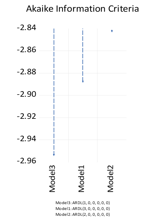
Figure 1: Optimal Lag to ARDL Model of GPD

Table 1: Descriptive Statistics of Research Variables

Table 2: Stationarity Test of Variables by Dickey-Fuller Test

a,b,c  at level, intercept, trend and intercept respectively. *: Significant at 5%

Table 3: ARDL Bounds Test Analysis of Models 

*: Significant at 5%

Table 4: ARDL Cointegration Long and Short Run Coefficients of Model 1

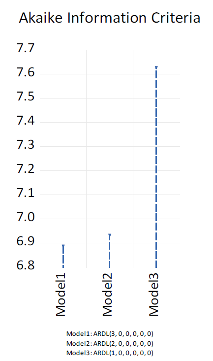
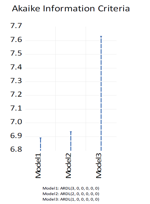
Figures 1 to 3 display the process of selecting optimal lag lengths for the ARDL models addressing GDP, FDI, non-oil GDP growth, and budget defilict. For this selection, widely recognized information criteria were applied—namely, the Akaike Information Criterion (AIC), Schwarz Bayesian Criterion (SBC), and Hannan–Quinn Criterion (HQC).

Table 5: ARDL Cointegration Long and Short Run Coefficients of Model 2

Table 6: ARDL Cointegration Long and Short Run Coefficients of Model3

Table 7: ARDL Diagnostic Test Results of Models

Table 3 reports the results of the ARDL bounds test, which assesses the existence of a long-run relationship—commonly referred to as cointegration—among the variables across all three models. For Model 1, the F-statistic is 28.07*, a value that substantially exceeds the upper bound critical values at all conventional significance levels, providing robust evidence in favor of cointegration. The t-Bounds test for Model 1 similarly yields a t-value above the upper bound, further supporting the presence of a stable long-run relationship.Model 2 demonstrates comparable results, with an F-statistic of 20.681*, surpassing the relevant I(1) critical values at the 5% significance level. The t-values confirm this finding, indicating cointegration among the examined variables. Model 3 follows this trend, with an F-statistic of 89.774* and t-Bounds test results that affirm statistical significance. Collectively, these findings indicate that all three models exhibit strong evidence of long-run relationships among their respective variables.

Figure2: Optimal Lag to ARDL Model of Non-oil GDP GrowthI

Figure3: Optimal Lag to ARDL Model of Budget Deficit

Table 4 provides the ARDL cointegration analysis for Model 1, highlighting both the long-run and short-run dynamics influencing GDP. In the long run, the coefficient for the lagged dependent variable (lGDP(-1)) is negative (-0.3639), suggesting a tendency for GDP to move back toward equilibrium after disturbances. While this adjustment is only marginally significant (p = 0.0632), it still points to some mean-reverting behavior in the series. Among the explanatory variables, both the exchange rate (-0.00026, p = 0.0372) and the interest rate (-0.00458, p = 0.036) display significant negative effects on GDP, indicating that currency depreciation and rising borrowing costs are associated with reductions in economic output. Other factors—including global oil prices, government oil revenues, and total public spending exhibit either positive or negative coefficients, but none of these relationships are statistically significant in the long run, implying a limited influence within the context of this model. The constant term is both positive and significant (1.118, p = 0.01), representing the baseline level of GDP in the absence of other influences. In the short run, the error correction term (CointEq(-1)*) is highly significant (-0.3639, p = 0.001), indicating that approximately 36% of deviations from the long-run equilibrium are corrected within one period. This finding supports the overall stability of the model. Furthermore, the model demonstrates robust explanatory power, as evidenced by an R-squared value of 0.995 and an F-statistic of 219.792 (p = 0.000), confirming that the ARDL specification effectively captures both short-term adjustments and long-term relationships among the variables.

Table 5 presents the ARDL cointegration results for Model 2, which investigates the factors influencing non-oil GDP growth. Notably, the lagged dependent variable, D(NON_OIL_GDP_GROWTH (-1)), is negative and highly significant (-1.584, p = 0.0041), suggesting a strong tendency for non-oil GDP growth to revert to its long-run equilibrium following disturbances. Essentially, any deviations are corrected rather quickly. Among the explanatory variables, the exchange rate stands out with a significant negative coefficient (-0.3427, p = 0.0322), indicating that currency depreciation has a detrimental effect on non-oil GDP growth. The impact of global oil prices is also negative (-0.997, p = 0.071), though only marginally significant. Government oil revenues, while displaying a positive coefficient (2.125, p = 0.115), do not reach conventional levels of statistical significance. Similarly, total public spending and interest rates exhibit either negative or negligible coefficients, and neither proves to be significant in the long run, implying their limited influence on non-oil GDP growth.The constant term is large and statistically significant (406.261, p = 0.0232), reflecting the baseline level of non-oil GDP growth when all explanatory variables are held at zero.In the short run, the second lag of non-oil GDP growth, D(NON_OIL_GDP_GROWTH(-2),2), shows a significant negative effect (-0.1005, p = 0.0309), highlighting short-term adjustment dynamics. The error correction term, CointEq(-1), is highly significant (-1.584, p = 0.000), which confirms that deviations from the long-run equilibrium are rapidly corrected, supporting the stability of the model. Overall, the model demonstrates substantial explanatory power, with an R-squared of 0.953 and a significant F-statistic (10.041, p = 0.020), both of which underscore the robustness of the identified relationships in both the short and long run.

Table 6 offers a detailed look at both the long-term and short-term behavior of Model 3. To start, the lagged budget deficit from the previous period shows a significant negative relationship with the current budget deficit, suggesting that past deficits tend to dampen current ones over time—a finding that departs from what one might intuitively expect. Turning to oil-related variables, both global oil prices and government oil revenues exhibit strong positive coefficients in the long run. This implies that increases in these variables contribute to expanding budget deficits, raising questions about fiscal management during periods of higher oil income. Meanwhile, total public spending displays a notable negative long-run effect, indicating that, contrary to some expectations, greater government spending is associated with a reduction in the deficit. Exchange rate and interest rate factors both emerge as positive and statistically significant, further amplifying the deficit. Looking at the short-run dynamics, the error correction term is negative and highly significant, confirming not only the presence of a stable long-run equilibrium but also that about 93.8% of any deviation from this equilibrium is corrected each period—a rather swift adjustment process. From a statistical perspective, the model demonstrates robust explanatory power, as reflected by an R-squared of 0.985 and a noteworthy F-statistic. These values underscore the overall reliability and significance of the estimated relationships within the model.

Diagnostic Tests 

Table 7 presents the outcomes of the ARDL diagnostic assessments for all three models, and, honestly, the results are pretty reassuring. The Breusch-Godfrey serial correlation LM test shows that serial correlation isn't an issue at all F-statistics across Models 1 to 3 are insignificant, so the models aren’t plagued by autocorrelation. Moving on, the Breusch-Pagan-Godfrey test doesn’t flag any heteroscedasticity, which means the error variances are stable and not acting up. The Jarque-Bera test also steps in to confirm that the residuals are normally distributed, which really strengthens the validity of the estimations. As for the Ramsey RESET test, it finds no evidence of misspecification, suggesting that the models are specified properly. Taken together, these diagnostic checks indicate the ARDL models are statistically sound, well-fitted, and robust, providing a solid foundation for empirical analysis.

The evidence is pretty clear: Iraq’s economic fortunes are tightly bound to the ups and downs of global oil prices, government oil revenues, and public spending. This isn’t just a theory it’s right there in the data. The ARDL models show a solid long-term connection between major economic indicators like GDP, non-oil GDP growth, and the budget deficit, and core influences such as oil revenues, spending strategies, shifts in the exchange rate, and interest rates. Basically, when oil prices get shaky, Iraq’s fiscal health and economic growth get shaky too.

The results highlight the country’s vulnerability to external shocks in oil markets, but there’s a bit of a silver lining: in the short run, the economy tends to adjust back toward equilibrium relatively quickly, showing at least some degree of resilience. Diagnostic checks back up the reliability of these models—no suspicious patterns, no odd errors. Bottom line: Iraq’s economic troubles aren’t some random bad luck. They’re a direct result of overreliance on oil, not enough economic diversification, and an unpredictable policy environment. If Iraq wants real, lasting stability, it needs to double down on structural reforms, smarter fiscal management, and genuine investment in non-oil sectors. Otherwise, it’s just more of the same old cycle.

Recommendations

• Diversification Beyond Oil: Iraq urgently needs to diversify its economy, shifting significant investment toward agriculture, manufacturing, renewables, and the service sector. Overreliance on oil revenues has repeatedly exposed the country to external price shocks; broadening the economic base could cushion Iraq from global market volatility and support more stable, sustainable growth

• Strengthening Fiscal Discipline: Fiscal policy should become more counter-cyclical, with the government establishing sovereign wealth or stabilization funds to save surplus oil revenue during boom cycles. These reserves would serve as a buffer, allowing Iraq to maintain essential public spending and limit deficits during inevitable downturns in oil prices

• Enhancing Monetary and Exchange Rate Stability: The Central Bank’s continued efforts to stabilize the exchange rate and contain inflation remain crucial. Effective coordination between fiscal and monetary authorities is indispensable, as policy misalignment can amplify economic instability rather than mitigate it

• Improving Public Spending Efficiency: Given the outsized role of public expenditure in Iraq’s economic activity, reforms are necessary to ensure more efficient budget allocations. Prioritizing investments in infrastructure, education, healthcare, and technology can drive long-term productivity gains, rather than fueling only short-term consumption

• Strengthening Institutions and Governance: Institutional reforms aimed at greater transparency, reduced corruption, and improved policy execution are essential. Stronger governance not only improves management of oil revenues but also fosters foreign investment and enhances overall stability

• Promoting Non-Oil Private Sector Development: Finally, cultivating a robust non-oil private sector requires regulatory reform, improved access to credit for small and medium enterprises, and expanded public–private partnerships

• Iraq urgently needs to strengthen its approach to economic risk management by moving beyond reactive measures. The country would benefit from implementing robust early warning systems to monitor the unpredictable fluctuations of oil prices

1. Caprio G. and Klingebiel D. "Bank insolvency: bad luck bad policy or bad banking?" In M. Bruno and B. Pleskovic (eds.) Annual World Bank Conference on Development Economics, 1996.

2. World Bank Group. "Iraq economic monitor: from war to reconstruction and economic recovery." World Express Inc., 2018, pp. 1–40.

3. MoP-Iraq. "National development plan 2018–2022." Ministry of Planning Iraq, 2018, pp. 1–38.

4. Central Statistical Organization. "Statistical indicators on the economic and social situation in Iraq 2012–2016." Ministry of Planning Iraq, 2018, pp. 1–36.

5. Larus J.R. and Ball T. "Rewriting executable files to measure program behavior." Software: Practice and Experience, vol. 24, no. 2, 1994, pp. 197–218.

6. Felton A. and Reinhart C. "First global financial crisis of 21st century." Vox EU Books, London, 2008.

7. Kotz D.M. "The financial and economic crisis of 2008: a systemic crisis of neoliberal capitalism." Review of Radical Political Economics, vol. 41, no. 3, 2009, pp. 305–317.