One of the most consumed vegetables around the world is tomatoes. Based on Food and Agriculture Organization (FAO), 170 million tons were produced worldwide [1]. Tomato's harvested area occupied 12.4 million acres of farmland globally. On the other hand, production had increased considerably. Between 2000 and 2014, production increased by 54% [1]. Based on Guan et al. [2], China, the United States, India, European Union and Turkey are top-five producers in the tomato market. The supply of those significant players forms 70% of tomato supply around the world.

In the Middle East, North African (MENA) region, Turkey, Iran and Jordan occupy the most significant pie share of tomato production [3]. According to [4], the production of the top three countries we just mentioned is 12 million tons for Turkey, 6.6 million tons for Iran and 864 thousand tons. The share of those three countries counts for 89% of total production in the MENA region. 

Even though we have three countries leading the production within the MENA region, harvested area and domestic demand had a significant gap between them. Figure 1 shows the trend of harvested area for Turkey, Iran and Jordan compared to the population of these three countries.

Ceteris Paribus, the growth in tomato demand is greater than the growth rate of the harvested area, with an increased gap between the two. This gap expansion is fueling policymakers' concerns about MENA food insecurity. This gap formed because the supply of local production is insufficient to consistently meet the needs of increased demand. 

In Turkey, literature has been conducted on analyzing economically different vegetables and fruits. Examples would be studies that analyzed the economic efficiency of dry apricot Gündüz et al. [5], kiwiGökdoğan [6], pumpkin Oğuz et al. [7] wheat and sunflower Unakıtan and Aydın [8] and Altaie [9], peach and cherry Aydın and Aktürk [10], pomegranate Ozalp et al. [11] and pear Aydın et al. [12]. On the other hand, some literature has been concerned with the economic analysis of tomato production in Turkey such as Yenihebit et al. [13], Akdogan [14], Weldegiorgis et al. [15] and Yelmen et al. [16]. In Iran and Jordan, literature that tackle the economic efficiency of tomato are inconclusive. Examples would be such as Hesampour et al. [17], Hasanshahi [18] and Raheli et al. [19]. Literature in technical efficiency in other MENA countries are Hassan [20,21,22,23] and Frhan [24]. However, to the author's knowledge, no study assessed tomato productive efficiency of those three countries in MENA region using Data Envelopment Analysis (DEA) employing the jackknife technique. 

Figure 1: Tomato harvested area and population in Turkey, Iran and Jordan between (1961 and 2019)

Analysis in this piece can benefit policymakers navigating through different initiatives to increase food security level. By demonstrating the use of standard methodologies to an empirical agricultural problem, this work contributes to the burgeoning literature in efficiency economics.

The aims of this piece are put together to show the source of inefficiency in tomato production at a macroeconomic level. This paper aims to:

Measuring technical efficiency (i.e. Overall Technical Efficiency (OTE), Pure Technical Efficiency (PTE) and Scale Efficiency (SE)) for each country. This can demonstrate how these countries can improve their performance or efficiency. 

Testing Technical Efficiency Scores Stability

The efficiency of tomato production in Turkey, Iran and Jordan can be considered an effective way to improve food security in the MENA region. Comparing the productive efficiency of tomatoes in these three countries can show strategies that may enhance the domestic production of tomatoes.

This study investigated factors affecting tomato production in the biggest producers in the MENA region. Those countries are Turkey, Iran and Jordan. Data utilized in this study were obtained from FAOSTAT. More specifically, data between 1961 and 2020 were used to study the economic analysis of the production of tomatoes. 

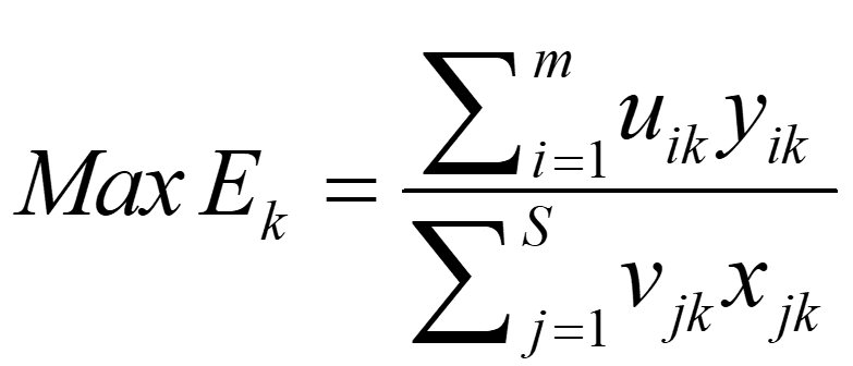
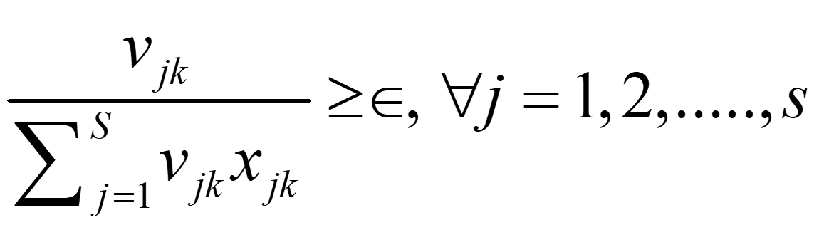
For the empirical part of this study, data envelopment analysis is used. More specifically, the jackknife technique will be followed to provide a robust, trusted and stable inquiry into the problem being studied. The following mathematical framework was used in the calculation of technical efficiency scores Mahajan et al. [25]:

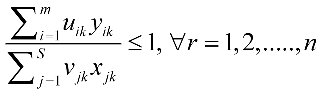
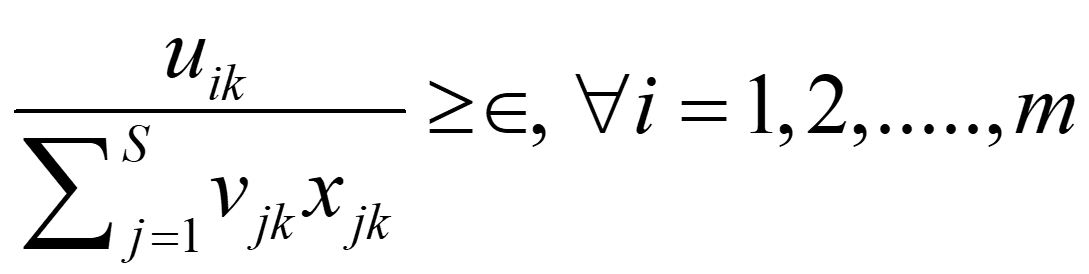
Subject to:

where:

y_ik    =  The i-th output produced by the k-th DMU

x_jk      =   The j-th input used by the k-th DMU

u_ik   =  The weight is given to input 

v_jk    =  The weight given to output 

n      =  The number of DMUs

m     =  The number of the output

s      =  Outputs number

Π    =  A constant value and very small

                In the above expression, the goal is to find values of u_ik and v_jk to maximize the efficiency of the k-th DMU. This is subject to a constraint that all efficiency measures must be£1. This expression is hard to solve. One way to solve it is to rely on a linear programming model called multiplier form. So, in order to estimate technical efficiency scores based on VRS, a convexity constraint

 (i.e. .) need to be imposed to get technical efficiency scores for the k-th firm. Based on what was just mentioned, an equivalent envelopment form can be derived by the following duality in linear programming. 

Factors affecting production and technical efficiency scores of tomato production in Turkey, Iran and Jordan are divided into standard production factors and sociodemographic variables related to climate change factors. Standard production factors are used in the first stage, while sociodemographic and variables related to climate change factors are used in the second. Variables in the first stage consist of area harvested, as a dependent variable, population (1000 person), yield (hg/ha), arable land (%), nitrogen nutrient (tonnes), phosphate nutrient (tonnes) and potash nutrient (tonnes). The second stage analysis consists of export values of tomato (1000 USD), gross production value (1000 USD), index of gross per capita production (number), emission of CH4, emission of N2O and emission of CO2. Also, trend analysis was utilized to determine the trend of the population in Iran, Jordan and Turkey and the trend of the harvested area in previously mentioned countries for the period of 1961-2020.

In this section, technical efficiency scores are reported. These are the Overall Technical Efficiency score (OTE), pure technical efficiency score and scale efficiency. After showing the previous score, efficiency scores and stability using the jackknife technique are shown and explained. 

Technical Efficiency Score Analysis

One important thing worth mentioning is that the efficiency scores shown here are relative efficiency scores. That means efficient years (with technical efficiency score =1) are used as a benchmark. In other words, efficiency scores are calculated relative to an efficient frontier. 

The CCR model was adopted first to calculate the technical efficiency score. However, the CCR model utilized Constant Return to Scale (CRS), where Scale Efficiency (SE) will not be considered. Based on that, pure technical efficiency is going to be assessed. The process of assessing is all around using the BCC model. This model will be followed to know the source of inefficiency, whether it is based on production inefficiency or the firm size. This is the definition of pure technical efficiency which means that it is that kind of efficiency that is attributed to the efficient exploitation of inputs taking into account the firm's size represented by scale size. Table 1 shows DEA results using the specification described above for Iran.

Out of 59 years, one is found to be overall technically efficient. Seven firms are technically efficient (BCC score = 1), i.e., they can reduce their excess inputs being utilized while maintaining the same output level. In comparison, the remaining 52 firms are relatively inefficient (BCC scores <1). PTE measures how efficiently inputs are converted into output(s) irrespective of the size of the firms. The average PTE is set to be 0.91, which means that given the operation scale, firms can reduce their inputs by 9 per cent of their observed levels without affecting output levels.

The results in Table 1 show that 1967, 1975, 1991, 2017, 2018 and 2019 are technically inefficient with CCR but efficient with BCC. This demonstrates unequivocally that businesses in these years can convert their inputs into outputs with 100% efficiency, but their OTE is poor because of the low scale efficiency score. 

Scale Efficiency (SE) can measure if the firm's size affects its efficiency score. In order to calculate scale efficiency, you need to divide the efficiency score obtained by CCR by the same score obtained by BCC. Getting a value of scale efficiency equals one means the firm operates at an optimal scale. Value of scale efficiency less than one means the firm is not operating at its optimum scale. 

Table 1: Technical efficiency scores with CRS and VRS of Iran between (1961-2019)

Results show that out of 59 years, four years are scale efficient while the remaining 55 years are scale inefficient. The average SE is 0.68, indicating that an average firm in these years may be able to decrease its inputs by 32 per cent beyond its best practice targets under VRS if it operated at CRS. 

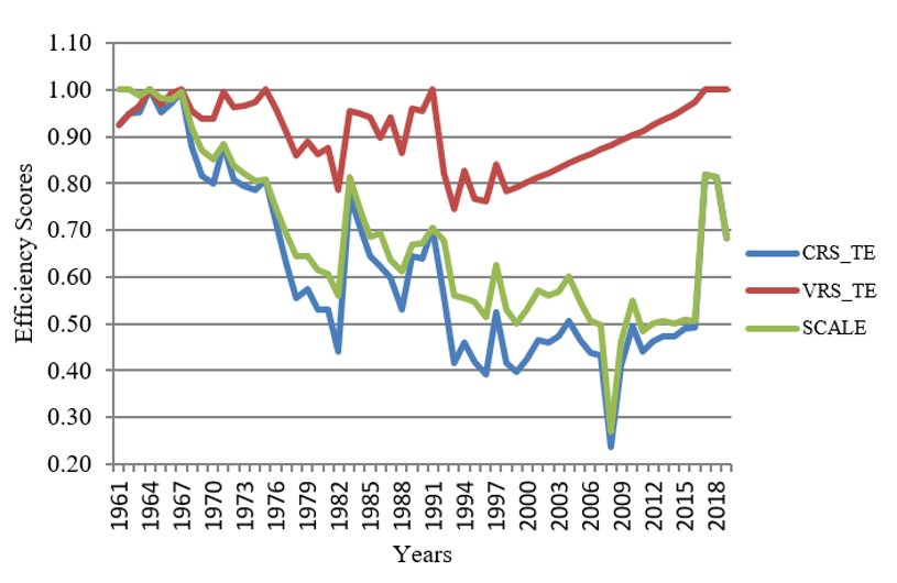
Figure 2: Trend of technical efficiency scores following CRS, VRS and SE of Iran between (1961-2019)

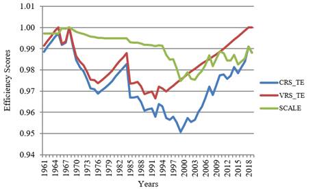
Figure 3: Depicts the trend of technical efficiency scores following CRS, VRS, and SE of Turkey between (1961-2019)

Figure 2 shows the trend of TEs over 59 years. Quick skimming over the figure shows that TE with VRS is decreasing at decreasing rate except in 2016, when things started to get back on track. In 2018, things started to get worse and this is concerning that this decrease might continue.

Moving on to Turkey. Table 2 shows technical efficiency scores with CRS and VRS in Turkey between (1961-2019). From the whole study sample, three are found to be overall technically efficient and nine years are pure technically efficient (BCC score = 1). In comparison, the remaining 50 years are relatively inefficient (BCC scores <1). The average PTE is set to be 0.98, which means that given the operation scale, firms can reduce their inputs by 2 per cent of their observed levels without affecting output levels.

The results in Table 2 show that 1963, 2015, 2016, 2017, 2018 and 2019 are technically inefficient with CCR but efficient with BCC. This demonstrates unequivocally that businesses in these years can convert their inputs into outputs with 100% efficiency, but their OTE is poor because of the low scale efficiency score. 

Results show that out of 59 years, 16 years are scale efficient while the remaining 43 years are scale inefficient. The average SE is 0.99, indicating that an average firm in these years may be able to decrease its inputs by 1 per cent beyond its best practice targets under VRS if it operated at CRS.

Figure 3 shows Turkey's trend of TEs and scale efficiency between 1961 and 2019. The same story is repeated here, similar to Iran. Technical efficiency when using VRS has significant volatility. The trend of VRS-TE decreased until 1992 when things started to improve.

Jordan’s TE scores are depicted in Table 3. This table depicts technical efficiency scores with CRS and VRS in Jordan. Between 1961 and 2019, one year is found to be overall technically efficient and four years are pure technically efficient (BCC score = 1), while the remaining 55 years are found to be relatively inefficient (BCC scores <1). 

Table 2: Technical efficiency scores with CRS and VRS of Turkey between (1961-2019)

The average PTE is set to be 0.89, which means that given the operation scale, firms can reduce their inputs by 11 per cent of their observed levels without affecting output levels.

Table 3 shows that 1963, 2015, 2016, 2017, 2018 and 2019 are technically inefficient with CCR but efficient with BCC. This demonstrates unequivocally that businesses in these years can convert their inputs into outputs with 100% efficiency, but their OTE is poor because of the low scale efficiency score. 

Table 3: Technical efficiency scores with CRS and VRS of Jordan between (1961-2019)

Results show that out of 59 years, 16 years are scale efficient while the remaining 43 years are scale inefficient. The average SE is 0.99, indicating that an average firm in these years may be able to decrease its inputs by 1 per cent beyond its best practice targets under VRS if it operated at CRS.

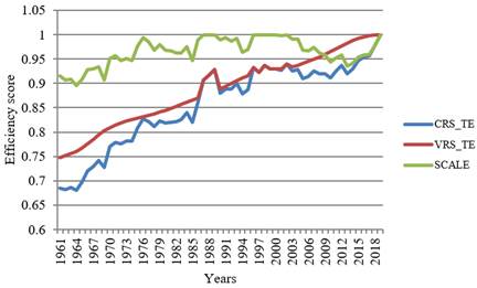
Figure 4: Trend of technical efficiency scores following CRS, VRS, and SE of Jordan between (1961-2019)

Table 4: Karl Person correlation coefficient with Jackknifing analysis using Pure Technical Efficiency (PTE) scores

Note: Numbers in parenthesis are p-value, and 58 is the sample size. 

Table 5: Correlation coefficients of Spearman rank of Jackknifing analysis using (PTE) scores 

Note: Numbers in parenthesis are p-value

Table 6: Karl Person correlation coefficient with Jackknifing analysis using Pure Technical Efficiency (PTE) scores

Note: Numbers in parenthesis are p-value, and 58 is the sample size. 

Table 7: Correlation coefficients of Spearman rank of Jackknifing analysis using (PTE) scores 

Note: Numbers in parenthesis are p-value

Table 8. Karl Person correlation coefficient with Jackknifing analysis using pure technical efficiency (PTE) scores

Note: Numbers in parenthesis are p-value, and 58 is the sample size. 

Table 9: Correlation coefficients of Spearman rank of Jackknifing analysis using (PTE) scores 

Note: Numbers in parenthesis are p-value

Jackknife Analysis or Stability Testing of Efficient Years

When testing for stability, we need to drop the highest efficient years with the most enormous peer count. This was done utilizing Pure Technical Efficiency scores or (PTE) obtained by VRS. This has to be done one at a time. In other words, you need to remove the most efficient first year and run DEA, then remove the second-highest efficient year, perform DEA and so on. This was done for Iran, Turkey and Jordan, respectively. This was done to test if outliers can affect technical efficiency scores and efficiency frontier. This procedure, known as Jackknifing, is based on Mostafa [26] and Ramanathan [27], whom they imposed a procedure testing the robustness of the results of DEA when outliers existed. Joshi and Singh [28] also follows the dropping of efficient firms with the most peer account. 

In Iran, three years got the highest peer count. Those years are 1991, 2006 and 2018. For Turkey, the story is different. Four years recorded the highest number of peer counts. Those years are 1984, 2016, 2017 and 2018. Finally, the highest peer count in Jordan was 1988, 1989, 2015 and 2019. Those years were dropped one at a time and each time DEA scores were recalculated for each country (Figure 4). 

After getting all technical efficiency scores, with Jackknifing technique and measuring efficiency change and years ranking, calculating the Spearman and Karl Pearson correlation coefficient of PTE scores need to be performed. 

Spearman and Pearson coefficients of correlation are depicted in Tables 4 and 5, respectively.

What can be inferred from Person correlation coefficients is that they ranged from 0.822 to 0.979 at a 5 per cent level of significance. This implies that the efficiency scores are still stable even with excluded most efficient years. Same story with Spearman correlation. Table 5 shows that correlation coefficients range from 0.862 to 0.959. This is an indicator that ranking years are also stable.

Tables 6 and 7 for Turkey show Pearson and Spearman correlation coefficients.

For Turkey, the story here is a little different. Person correlation coefficients ranged from 0.735 to 0.999 at a 5 per cent significance level. However, when excluding 2018, efficiency scores became unstable. For Spearman rank correlation, it ranged between 0.757 and 0.999. With this ranking correlation, an unstable rank was approved when the year 2018 was excluded. 

Tables 8 and 9 show Pearson and Spearman rank correlation for Jordan between 1961 and 2019.

The same scenario happened here compared in Turkey. When excluding the most efficient years, 2015 and 2019, one at a time, Karl Pearson correlation coefficients approved that efficiency scores became unstable. Also, Spearman rank correlation showed that the whole rank became unstable when excluding these two most efficient years.

This work use panel data of the top three tomato producers within the MENA region between 1961 and 2019. For Iran, results showed that one year using CCR and seven years using BCC is recorded as technically efficient. However, one year in CCR and four years in BCC have shown efficiency for Turkey and Jordan. The remaining years within the three previously mentioned countries were operating far from the efficient frontier. The average pure technical efficiency was (0.91, 0.98 and 0.89) per cent for Iran, Turkey and Jordan, respectively. This means that, on average, these countries can reduce their input usage by (0.9, 0.2 and 0.11) per cent, respectively, without affecting their output level given their operation scale. This would also mean that those years are (0.91, 0.98, 0.89) per cent technically inefficient and (0.33, 0.1 and 0.4) scale inefficient due to lack of management performance. This suggests that in those years, improvements were possible. For Iran, jackknife analysis showed stability over technical efficiency scores when the most efficient years. The story is different for Turkey and Jordan. Results showed that technical efficiency scores are unstable when the most efficient years are excluded. This would strongly recommend that jackknife analysis is very crucial in efficiency analysis. This is because it pays strong attention to outliers since those can affect technical efficiency scores and affect policy extracted from those scores.

1. FAO STAT. FAOSTAT. 2022. https://www.fao.org/faostat/en/#data.

2. Guan, Z. et al. "The U.S. tomato industry: An overview of production and trade." EDIS, vol. 2018, no. 2, 2018, https://doi.org/10.32473/edis-fe1027-2017.

3. IndexBox. "Turkey emerges as the largest producer of tomatoes in the Middle East." Global Trade Magazine, 4 Mar. 2020, https://www.globaltrademag.com/turkey-emerges-as-the-largest-producer-of-tomatoes-in-the-middle-east/.

4. IndexBox. "Tomato market in the Middle East posted solid gains over the last decade." Global Trade Magazine, 22 Aug. 2020, https://www.globaltrademag.com/tomato-market-in-the-middle-east-posted-solid-gains-over-the-last-decade/.

5. Gündüz, O. et al. "Measuring the metafrontier efficiencies and technology gaps of dried apricot farms in different agro-ecological zones." [Include journal name if available], 2021.

6. Gökdoğan, O. "Energy and economic efficiency of kiwi fruit production in Turkey: A case study from Mersin Province." Erwerbs-Obstbau, 2022, pp. 1–6.

7. Oğuz, H.İ. et al. "Determination of the energy input-output analysis and economic efficiency of pumpkin seed (Cucurbita pepo L.) production in Turkey: A case study of Nevsehir province." [Include journal name if available], 2020.

8. Unakıtan, G. and Aydın, B. "A comparison of energy use efficiency and economic analysis of wheat and sunflower production in Turkey: A case study in Thrace Region." Energy, vol. 149, 2018, pp. 279–285.

9. Altaie, K. "Three essays on wheat production efficiency in Iraq: Comparison between MENA countries and internal comparison of districts." Colorado State University, 2019.

10. Aydın, B. and Aktürk, D. "Energy use efficiency and economic analysis of peach and cherry production regarding good agricultural practices in Turkey: A case study in Çanakkale province." Energy, vol. 158, 2018, pp. 967–974.

11. Ozalp, A. et al. "Energy analysis and emissions of greenhouse gases of pomegranate production in Antalya province of Turkey." Erwerbs-Obstbau, vol. 60, no. 4, 2018, pp. 321–329.

12. Aydın, B. et al. "Comparative profitability and productivity analysis in dwarf pear production in Turkey: Case of Bursa Province." Custos e Agronegocio On Line, vol. 15, no. 1, 2019, pp. 397–416.

13. Yenihebit, N. et al. "An efficiency assessment of irrigated tomato (Solanum lycopersicum) production in the Upper East Region of Ghana." Journal of Development and Agricultural Economics, vol. 12, no. 1, 2020, pp. 1–8.

14. Akdogan, A. "Data envelopment analysis and an application in the tomato sector in Turkey." PhD thesis, Washington State University, 2019.

15. Weldegiorgis, L.G. et al. "Resources use efficiency of irrigated tomato production of small-scale farmers." International Journal of Vegetable Science, vol. 24, no. 5, 2018, pp. 456–465.

16. Yelmen, B. et al. "Energy efficiency and economic analysis in tomato production: A case study of Mersin province in the Mediterranean region." Applied Ecology and Environmental Research, vol. 17, no. 4, 2019, pp. 7371–7379.

17. Hesampour, R. et al. "Technical efficiency, sensitivity analysis and economic assessment applying data envelopment analysis approach: A case study of date production in Khuzestan State of Iran." Journal of the Saudi Society of Agricultural Sciences, vol. 21, no. 3, 2022, pp. 197–207.

18. Hasanshahi, M. "Measuring the effect of heavy spring rainfall on technical efficiency of tomato production in Arsanjan." [Include journal name if available], 2019.

19. Raheli, H. et al. "A two-stage DEA model to evaluate sustainability and energy efficiency of tomato production." Information Processing in Agriculture, vol. 4, no. 4, 2017, pp. 342–350.

20. Hassan, F.A.M. "Data envelopment analysis (DEA) approach for assessing technical, economic and scale efficiency of broiler farms." Iraqi Journal of Agricultural Sciences, vol. 52, no. 2, 2021, pp. 291–300, https://doi.org/10.36103/ijas.v52i2.1290.

21. Al, A., et al. "Impact of herd size on the productive efficiency of sheep breeding projects at the Kokjali region in Nineveh Governorate for the production season 2018." Iraqi Journal of Agricultural Sciences, vol. 51, no. 6, 2020, pp. 1613–1622, https://doi.org/10.36103/ijas.v51i6.1188.

22. Lafta, A., et al. "Measuring the economic efficiency and total productivity of resource and the technical change of agricultural companies in Iraq using SFA and DEA for the period 2005-2017." Iraqi Journal of Agricultural Sciences, vol. 51, no. 4, 2020, pp. 1104–1117, https://doi.org/10.36103/ijas.v51i4.1089.

23. Al, K. and E. "Economical analysis of efficiency of rice farms in Al-Najaf Alashraf for the agricultural season 2017." Iraqi Journal of Agricultural Sciences, vol. 50, no. 2, 2019, https://doi.org/10.36103/ijas.v2i50.654.

24. Frhan, A.H. et al. "A comparative study of technical efficiency of certified wheat cultivars (ADNA 99 and IPA 99) in Iraq during the season 2014-2015: Wasit Governorate as a case study." Iraqi Journal of Agricultural Sciences, vol. 48, no. 6B, 2017, https://doi.org/10.36103/ijas.v48i6.

25. Mahajan, V. et al. "Technical efficiency analysis of the Indian drug and pharmaceutical industry: A non-parametric approach." Benchmarking: An International Journal, 2014.

26. Mostafa, M. "Benchmarking top Arab banks’ efficiency through efficient frontier analysis." Industrial Management and Data Systems, 2007.

27. Ramanathan, R. An introduction to data envelopment analysis: A tool for performance measurement. Sage, 2003.

28. Joshi, R.N. and Singh, S.P. "Technical efficiency and its determinants in the Indian garment industry." Journal of the Textile Institute, vol. 103, no. 3, 2012, pp. 231–243.